Generalized Ricker function — ricker • sdbuildR

Computes the generalized Ricker function, a smooth hump-shaped curve that rises from zero, peaks, and then decays back towards zero. It is commonly used to describe humped (non-monotonic) dependencies, such as stock-recruitment relationships in ecology or size-dependent predation.

Usage

ricker(x, location = 1, upper = 1, shape = 1, a = NULL, b = NULL)

Arguments

x: Value at which to evaluate the function. Because the curve involves a fractional power of x, x is expected to be non-negative.
location: Value of x at which the function reaches its peak. Defaults to 1.
upper: Maximal value (height) of the function, attained at the peak. Defaults to 1.
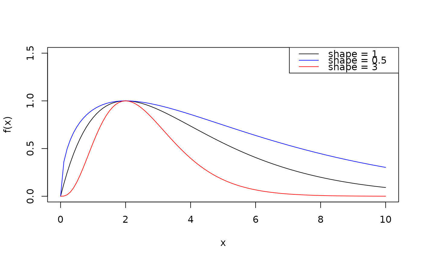
shape: Exponent controlling the width of the peak: values above 1 narrow the peak, values below 1 broaden it. shape = 1 gives the standard Ricker function. Defaults to 1.
a, b: Coefficients of the equivalent expanded form $f(x) = a \cdot x^{shape} \cdot e^{-b \cdot x}$. Optional alternative to location and upper: when both a and b are supplied, they take precedence and set location = shape / b and upper = a \cdot (location / e)^{shape}. With shape = 1 this is the standard Ricker parameterization $f(x) = a \cdot x \cdot e^{-b \cdot x}$. Supplying only one of them, or combining them with an explicit location or upper, is an error. Default to NULL.

Value

Numeric value given by $$f(x) = upper \cdot \left(\frac{x}{location} \cdot e^{1 - x / location}\right)^{shape}$$

Details

The generalized Ricker function (Persson et al., 1998) is defined as:

$$f(x) = upper \cdot \left(\frac{x}{location} \cdot e^{1 - x / location}\right)^{shape}$$

with a power parameter ($\alpha$, or shape) that broadens or narrows the peak. The function peaks at x = location, where it attains the value upper, for any shape.

Expanding the expression shows that it is equivalent to:

$$f(x) = a \cdot x^{shape} \cdot e^{-b \cdot x}$$

with coefficients

$$a = upper \cdot (e / location)^{shape}$$ $$b = shape / location$$

or equivalently

$$location = shape / b$$ $$upper = a \cdot (location / e)^{shape}.$$

Note that $e$ is the base of the natural logarithm (i.e., exp(1)). When shape = 1, the power on x is 1 and this reduces to the standard Ricker function $f(x) = a \cdot x \cdot e^{-b \cdot x}$, with $a = upper \cdot e / location$ and $b = 1 / location$.

See Bolker, B. M. (2008). Ecological Models and Data in R. Princeton University Press, Section 8.1.

Examples

ricker(1)
#> [1] 1

# Adjust parameters
ricker(2, location = 2, upper = 10, shape = 1)
#> [1] 10

# Use the expanded form f(x) = a * x^shape * exp(-b * x) instead.
# With shape = 1 this is the standard Ricker f(x) = a * x * exp(-b * x).
ricker(3, a = 2.5, b = 0.4)
#> [1] 2.258957
# equivalent to:
ricker(3, location = 1 / 0.4, upper = 2.5 * (1 / 0.4 / exp(1)))
#> [1] 2.258957

# The mapping holds for any shape, e.g. f(x) = a * x^2 * exp(-b * x)
ricker(3, a = 2.5, b = 0.4, shape = 2)
#> [1] 6.77687

# Visualize different peak widths
curve(ricker(x, location = 2), from = 0, to = 10, ylab = "f(x)", ylim = c(0, 1.5))
curve(ricker(x, location = 2, shape = 0.5), add = TRUE, col = "blue")
curve(ricker(x, location = 2, shape = 3), add = TRUE, col = "red")
legend("topright",
  legend = c("shape = 1", "shape = 0.5", "shape = 3"),
  col = c("black", "blue", "red"), lty = 1
)